In 1965 Jack Elton Bresenham published the paper Algorithm for computer control of a digital
plotter in the IBM Systems Journal, volume 4, number 1.
It explained how a line could be approximated on an integer grid.
The algorithm is still used today as a rasterization
technique for rendering lines on video displays or printers.
As Bresenham's paper suggests, however, it was originally devised for a
plotter, capable of moving from one grid point to one of
the adjacent eight grid points.
We consider drawing a line from (0,0) to (Δx,Δy) on an
integer grid by choosing the points that lie close to the true line. We also assume that
Δx>0 and Δx≥Δy≥0. The method is easily
extended to the general case with arbitrary starting and ending points.
The line has the form
y=f(x)=ΔxΔyx
and we aim to sample the line at the grid points (xk,yk) with xk=k for k=0,1,…,Δx and y0=0.
We now associate with each step an error term,
∇k=2Δx[f(xk)−(yk−1+21)]=2xkΔy−(2yk−1+1)Δx.
The interpretation of this error term is important: It expresses the difference at
x=xk between the line's true y-coordinate, f(xk), and the
midpoint between the previously chosen y-coordinate, yk−1, and its
successor, yk−1+1. The factor 2Δx is there to make all
quantities integral. The sign of ∇k is thus crucial:
If ∇k≤0 then yk=yk−1 lies closest to the line (it is a tie for ∇k=0).
If ∇k>0 then yk=yk−1+1 should be chosen.
Note how the magnitude of ∇k also tells exactly how far from the true line the
chosen grid point is. It is straightforward to show that −2Δx<∇k≤2Δx for k=1,2,…,Δx.
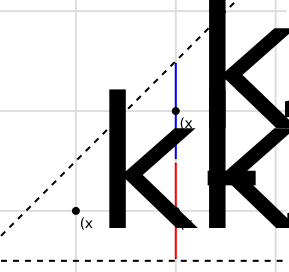
Figure 1. Given that the previous point is at (xk-1, yk-1),
the dashed lines indicate the two extreme cases for the line being approximated. ∇k
will be negative if the line goes through the red area and positive if it goes through the blue
area.
To determine the ∇k's we start with the base case:
∇1=2⋅1⋅Δy−(2⋅0+1)Δx=2Δy−Δx.
For k=1,2,…,Δx−1 we get
∇k+1−∇k=2(xk+1−xk)Δy−2(yk−yk−1)Δx.
We now split into the two cases for ∇k and get
∇k+1={∇k+2Δy∇k+2Δy−2Δxfor ∇k≤0,for ∇k>0,
for k=1,2,…,Δx−1.
These expressions determine all the ∇k's which, in turn, determines all the yk's.
Feel free to leave any question, correction or comment in this
Mastodon thread.