Series: Finite Element Method › Discrete

Continuous Galerkin

The previous post noted that both continuous and discontinuous Galerkin methods can be cast in the same element-by-element assembly framework. The defining difference is what happens at inter-element faces. In the continuous Galerkin method the discrete space satisfies $V_h \subset H^1(\Omega)$, which forces the global basis functions to be continuous across every shared face.

To see why this matters, recall that a function belongs to $H^1(\Omega)$ only if it is square-integrable together with its first derivatives. A piecewise-defined function that has a jump discontinuity along a face has an ill-defined derivative there — formally a Dirac delta contribution — and falls outside $H^1(\Omega)$. The weak formulation of elliptic problems requires test and trial functions in $H^1(\Omega)$, so a jump-discontinuous basis function would make the stiffness matrix entries $a(\phi_j, \phi_i)$ ill-defined. Continuity across faces is therefore not a convenience but a hard requirement.

The standard way to enforce continuity is through the Kronecker delta property of the shape functions. Nodes $x_1, \ldots, x_N$ are placed in the mesh — at vertices, and possibly also at edge midpoints or face centres depending on the element order — and the shape functions are required to satisfy

$$\phi_i(x_j) = \delta_{ij}, \qquad i, j = 1, \ldots, N.$$

This property has two immediate consequences. First, the discrete solution $u_h = \sum_j u_j\,\phi_j$ satisfies $u_h(x_i) = u_i$, so the unknown coefficients are simply the values of the solution at the nodes. Second, and more importantly for continuity, adjacent elements can enforce agreement across their shared face simply by sharing nodes.

Consider two triangular elements sharing an edge. The edge carries two endpoint nodes (for linear elements) or two endpoint nodes and a midpoint node (for quadratic elements). On each element, the restriction of any shape function to the shared edge is a polynomial, and that polynomial is uniquely determined by its values at the nodes on the edge. Because the shape functions on both elements satisfy the Kronecker delta property and refer to the same shared nodes, they agree at every node on the edge and therefore on the entire edge. No additional coupling condition needs to be imposed: continuity follows automatically from the shared node structure.

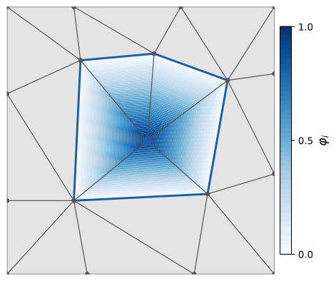
The figure below illustrates a piecewise-linear basis function $\varphi_i$ on a triangular mesh. The function equals one at the node $x_i$ and zero at all other nodes; within each element it varies linearly. The blue boundary marks the support of $\varphi_i$ — the union of all elements sharing $x_i$. Outside this patch the function is identically zero. Across every edge of the patch the function value transitions smoothly to zero, matching the zero values in the adjacent elements.

For this mechanism to work, the polynomial degree of the shape functions on a shared face must be the same on both sides, and the face must carry exactly the nodes needed to uniquely determine a polynomial of that degree. For linear triangles one node per edge endpoint suffices; for quadratic triangles a midpoint node must also be present and shared. This requirement drives the node placement rules that appear in each of the element posts that follow.