The Quad4 Element

The Quad4 element is the simplest quadrilateral element: 4 nodes, one at each corner of the reference square, with bilinear shape functions. The reference domain is $\hat{Q} = [0,1]^2$ with corners

\hat{x}_0 = (0,0), \quad \hat{x}_1 = (1,0), \quad \hat{x}_2 = (1,1), \quad \hat{x}_3 = (0,1),

matching the quadrilateral reference domain.

In the library, it is implemented in elements/quad4.py by the class Quad4.

The shape functions are obtained as tensor products of the two Line2 shape functions. Writing $\ell_0(t) = 1 - t$ and $\ell_1(t) = t$ for the linear Lagrange basis on $[0,1]$ , each Quad4 shape function takes the form $\ell_a(\hat{x})\,\ell_b(\hat{y})$ for appropriate choices of $a, b \in \{0,1\}$ :

N_0 = (1-\hat{x})(1-\hat{y}), \quad N_1 = \hat{x}(1-\hat{y}), \quad N_2 = \hat{x}\,\hat{y}, \quad N_3 = (1-\hat{x})\,\hat{y}.

Each $N_i$ equals one at its own corner and zero at the other three, and the four functions form a partition of unity. The figure below shows all four shape functions as filled contour plots over the reference square.

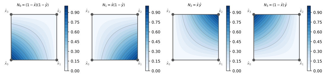
Shape functions of the Quad4 element

Unlike the triangular elements, the Quad4 shape functions are not linear polynomials — they are bilinear, meaning linear in each variable separately but containing the cross term $\hat{x}\hat{y}$ . As a result, the reference-domain gradients are not constant but depend on position:

\nabla N_0 = \begin{pmatrix}-(1-\hat{y})\\-(1-\hat{x})\end{pmatrix}, \quad \nabla N_1 = \begin{pmatrix}1-\hat{y}\\-\hat{x}\end{pmatrix}, \quad \nabla N_2 = \begin{pmatrix}\hat{y}\\\hat{x}\end{pmatrix}, \quad \nabla N_3 = \begin{pmatrix}-\hat{y}\\1-\hat{x}\end{pmatrix}.

Quad4 can represent any function of the form $a + b\hat{x} + c\hat{y} + d\hat{x}\hat{y}$ exactly. In particular it reproduces all linear functions, so the element achieves first-order accuracy. For the isoparametric mapping, the same four shape functions carry the reference square to any physical quadrilateral with vertices $x_0, x_1, x_2, x_3 \in \mathbb{R}^d$ via $F_e(\hat{x}) = \sum_{i=0}^3 x_i\,N_i(\hat{x},\hat{y})$ . When the physical element is not a parallelogram the mapping is genuinely nonlinear, which is why the Jacobian must be evaluated numerically at each quadrature point rather than once per element.