The Wave Equation on the Unit Square

Let us consider the wave equation

$$\frac{\partial^2 v}{\partial t^2} = \Delta v$$

on the unit square $\Omega = [0, 1] \times [0, 1]$ with homogeneous Dirichlet boundary conditions, $v|_{\partial \Omega} = 0$.

We would like to solve this partial differential equation numerically. First, we discretize in space using a finite difference discretization as described in a previous post. More specifically, we use $n$ interior points in each direction and a grid spacing of $h = 1/(n+1)$. We introduce the matrix $U \in \mathbb{R}^{n \times n}$ with entries $U_{ij} = v(ih,jh)$ for $i,j = 1,2,\ldots,n$. Finally, we set $u = \operatorname{vec}(U)$, where the $\operatorname{vec}$ operator stacks the columns of $U$ on top of each other. Thus, $u \in \mathbb{R}^{n^2}$.

We now have

$$\frac{\partial^2 u}{\partial t^2} = D u,$$

where $D = L \oplus L$ and $L \in \mathbb{R}^{n \times n}$ is the finite difference discretization of the Laplace operator:

$$L = \frac{1}{h^2} \begin{bmatrix} -2 & 1 & 0 & \cdots & 0 \\ 1 & -2 & 1 & \ddots & \vdots \\ 0 & 1 & -2 & \ddots & 0 \\ \vdots & \ddots & \ddots & \ddots & 1 \\ 0 & \cdots & 0 & 1 & -2 \end{bmatrix}$$

(see the previous post for the definition of $\oplus$ and other details).

So now we have a system of ordinary differential equations. It is of second order, however, but it is easily transformed into a system of first order ODEs:

$$\frac{\partial}{\partial t} \begin{bmatrix} u \\ u_t \end{bmatrix} = \begin{bmatrix} u_t \\ D u \end{bmatrix} = \begin{bmatrix} 0 & I \\ D & 0 \end{bmatrix} \begin{bmatrix} u \\ u_t \end{bmatrix}.$$

Now, given initial values for $u$ and $u_t$ at time $t=0$, we have a system that can be solved using a numerical ODE solver.

Let us now describe how to solve this system numerically using Python's numpy and scipy libraries.

First, the grid:

n = 199
h = 1 / (n + 1)
x = y = np.linspace(0, 1, n + 2)

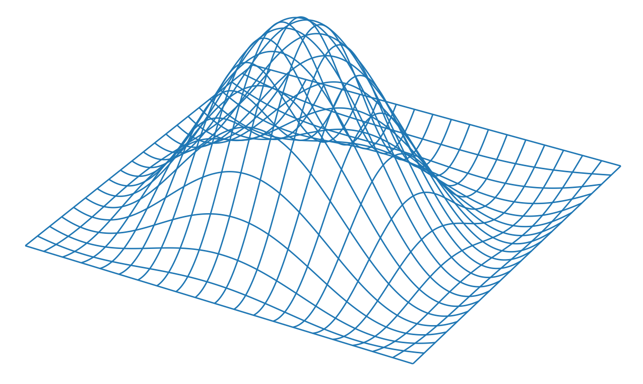
Next, the initial conditions:

X, Y = np.meshgrid(x, y)
R = np.sqrt((X - 0.45)**2 + (Y - 0.4)**2)
U = 20 * np.exp(-R**2) * np.cos(4 * R) * X * (1 - X) * Y * (1 - Y)

This expression for $U$ is chosen to have a nice, non-trivial shape and to satisfy the boundary conditions:

We now set up the Laplace matrix $L$ and its 2D version $D$:

L = (scipy.sparse.eye(n, k=-1) - 2 * scipy.sparse.eye(n)
     + scipy.sparse.eye(n, k=1)) / h**2
D = scipy.sparse.kronsum(L, L)

We set the initial values for $u(0)$ (a vector version of the inner of $U$), use $u_t(0)=0$ and set up the time range for the solver:

u0 = U[1:-1, 1:-1].reshape(-1)
ut0 = np.zeros_like(u0)
timespan = [0, 5]
sample_times = np.linspace(0, 5, 200)

The variable sample_times is used to instruct the solver to record the solution at these times.

Finally, we solve the system using scipy's initial value ODE solver, which uses the explicit Runge-Kutta method of order 5(4) by default:

R = scipy.integrate.solve_ivp(
    lambda _, u: np.concatenate((u[n*n:], D @ u[:n*n])),
    timespan,
    np.concatenate((u0, ut0)),
    t_eval=sample_times
)

By plotting each of the sampled solutions, we can view an animation of the solution:

(The plotting was done using matplotlib and the movie was created using ffmpeg.)